


How Automatic Temperature Control Systems Integrate with Smart Nozzles to Improve Cooling Precision
Table of Contents
- Introduction: Why Integration Matters for Cooling Precision
- Critical Temperature Control Parameters in Spray Cooling
- Smart Nozzle Technology: Real-Time Flow and Spray Adjustment
- Integration Architecture: Sensors, Controllers, and Actuated Nozzles
- Worked Example: Steel Billet Cooling Temperature Control
- Performance Comparison: Conventional vs. Integrated Smart Systems
- Common Integration Mistakes and Field Solutions
- FAQ
- Conclusion
1. Introduction: Why Integration Matters for Cooling Precision
In continuous steel rolling, semiconductor wafer processing, and data center thermal management, maintaining target temperature within ±2–5°C is not a luxury—it's a metallurgical or reliability requirement. Traditional fixed-flow spray cooling systems operate open-loop: they deliver a preset flow rate regardless of real-time thermal load. When product throughput varies, ambient temperature shifts, or upstream heating fluctuates, fixed systems either overcool (wasting water and energy) or undercool (risking quality defects or equipment damage).
Automatic temperature control systems integrated with smart nozzles close this loop. They continuously measure surface or process temperature, calculate the cooling duty gap, and modulate nozzle flow rate, spray angle, or droplet size in real time. From our field implementation data, integrated systems reduce temperature variance by 60–75% compared to manual setpoint adjustment, cut water consumption by 20–40% in variable-load applications, and extend nozzle service life by reducing unnecessary high-pressure operation.
This guide explains how automatic temperature control systems communicate with smart nozzles, which nozzle actuation methods work best for different cooling scenarios, and how to size, install, and troubleshoot integrated cooling systems. We focus on actionable design steps and real field data rather than theoretical overviews.
2. Critical Temperature Control Parameters in Spray Cooling
2.1 Cooling Rate and Heat Flux
Spray cooling removes heat through two mechanisms: convective heat transfer from the hot surface to the liquid film, and evaporative cooling from droplet vaporization. The cooling rate depends on:
- Flow rate per unit area (L/min/m²): Higher flow increases heat removal but also water usage.
- Droplet size (Dv0.5): Smaller droplets (50–200 microns) maximize surface area for evaporation; larger droplets (400–800 microns) deliver higher impact force and liquid film coverage.
- Impact velocity: Derived from nozzle pressure and spray angle—higher velocity improves film renewal but can cause splashing.
- Surface temperature and approach: The Leidenfrost point (typically 200–300°C for water on steel) defines the transition from nucleate boiling to film boiling. Below this, liquid contact is stable; above it, a vapor film insulates the surface and dramatically reduces cooling efficiency.
A common mistake is assuming that doubling flow rate doubles cooling rate. In reality, once the surface is fully wetted, additional flow provides diminishing returns. From our infrared thermal mapping, increasing flow from 10 L/min/m² to 20 L/min/m² on a 600°C steel plate improves cooling by ~40%, not 100%, because film thickness reaches a transport-limited regime.
2.2 Temperature Uniformity and Gradient Control
In applications like continuous casting or heat treatment, local temperature gradients cause thermal stress and warping. Spray uniformity—how evenly droplets distribute across the target—is as critical as total flow rate. Uniformity is quantified by the coefficient of variation (CV) of water distribution measured on water-sensitive paper or patternator grids.
Smart nozzles improve uniformity through:
- Variable spray angle adjustment: Widening the cone when the target is closer, narrowing when farther.
- Zoned flow control: Independently modulating nozzle groups in multi-zone cooling beds.
- Pulsed spray: Alternating nozzles on/off in millisecond cycles to smooth instantaneous coverage.
Automatic control systems measure temperature at multiple points (typically 3–9 thermocouples across the cooling zone) and calculate local heat flux imbalances. The controller then adjusts individual nozzle flows or pressures to flatten the temperature profile.
2.3 Response Time and System Lag
Temperature control precision is limited by system lag—the delay between sensor detection and cooling response. Major lag sources include:
- Sensor lag (0.5–3 seconds): Thermocouples embedded in product or non-contact pyrometers averaging over a spot size.
- Controller computation lag (0.1–0.5 seconds): PID loop calculation and communication to actuators.
- Valve actuation lag (0.3–2 seconds): Pneumatic or stepper-motor valves moving from one position to another.
- Hydraulic lag (0.2–1 second): Pressure wave travel time through piping from valve to nozzle.
- Thermal diffusion lag (2–10 seconds): Heat conduction from the measurement point to the cooled surface layer.
Total system lag of 3–15 seconds is typical. For fast-moving product (e.g., steel strip at 5 m/s), a 5-second lag means the control action applies 25 meters downstream from where temperature was measured. Advanced systems use predictive feedforward control—estimating future temperature based on product speed, upstream heating, and known cooling curves—to compensate for lag.
3. Smart Nozzle Technology: Real-Time Flow and Spray Adjustment
3.1 Actuation Methods: Pressure Modulation vs. Mechanical Flow Control
Smart nozzles adjust cooling output through three main methods:
| Actuation Method | Mechanism | Flow Range | Response Time | Pressure Stability | Typical Cost Multiplier |
|---|---|---|---|---|---|
| Pressure modulation (servo valve) | Upstream proportional valve adjusts supply pressure; nozzle flow follows Q = k√P | 10:1 turndown | 0.3–1 sec | Poor (pressure ripple affects other nozzles on same manifold) | 1.5–2x |
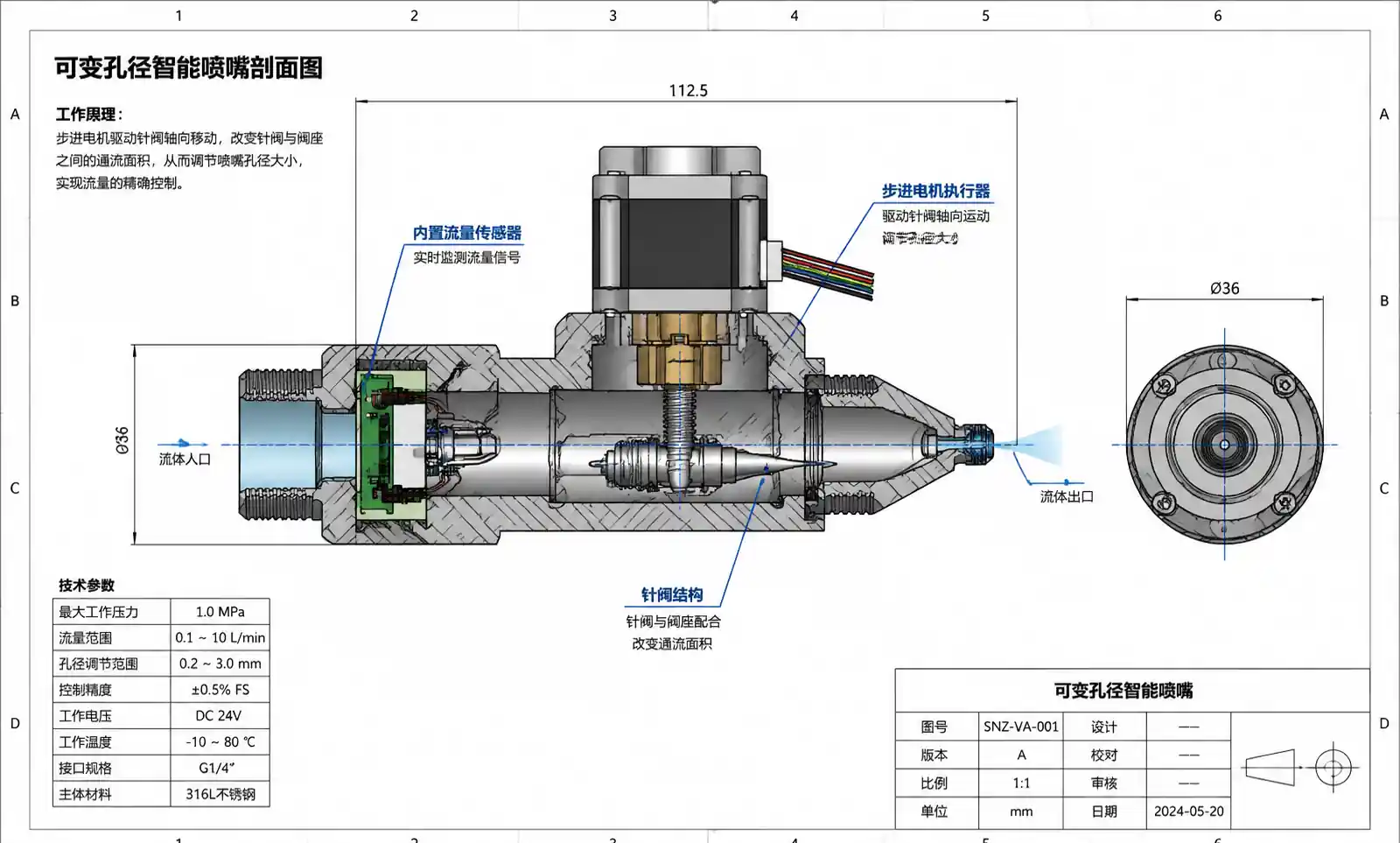
| Variable orifice (needle valve) | Internal needle retracts or advances into orifice | 20:1 turndown | 0.5–2 sec | Excellent (independent of supply pressure) | 3–5x |
| Rotary vane or iris | Mechanical vane rotates to change effective orifice area | 15:1 turndown | 0.8–2 sec | Excellent | 4–6x |
| On/off pulsed (solenoid) | Rapid cycling (10–50 Hz) with variable duty cycle | 100:1 effective | 0.05–0.2 sec per pulse | Excellent (fixed operating pressure) | 1.2–1.8x |
Pressure modulation is the simplest and cheapest but suffers from cross-talk: changing pressure for one nozzle affects all others on the manifold. It works well for single-zone or grouped control but not for individual nozzle modulation.
Variable orifice nozzles use a stepper motor or piezoelectric actuator to move an internal needle. They provide true independent control and maintain constant spray angle and droplet size across the flow range. However, the actuator adds mechanical complexity and potential wear points. From our wear testing in steelmaking environments, actuator seals last 8,000–15,000 hours in clean water but only 2,000–5,000 hours in recycled scale-laden water—filtration to <100 microns is mandatory.
Pulsed on/off nozzles are emerging as a cost-effective alternative. A fast solenoid valve cycles the nozzle on/off at 20–50 Hz, and the controller varies the duty cycle (percentage of time open) to achieve the desired average flow. At 50 Hz with 20% duty cycle, the nozzle is open for 4 ms every 20 ms. Because the nozzle operates at fixed pressure when open, spray characteristics remain constant. The human eye perceives frequencies above ~15 Hz as continuous, so pulsed spray appears steady. This method provides excellent turndown (up to 100:1), fast response, and avoids valve throttling wear. The trade-off is potential fatigue on solenoid springs and seats—high-quality solenoids rated for 50 million cycles are recommended.
3.2 Integrated Sensors and Feedback
True "smart" nozzles embed sensors directly in the nozzle body or mounting block:
- Flow meters (turbine or magnetic): Measure actual flow rate to detect clogging or orifice wear. A 20% flow drop at constant pressure indicates orifice enlargement from wear.
- Pressure transducers: Monitor local pressure to verify valve commands and detect manifold blockages.
- Temperature sensors (thermocouples or RTDs): Measure coolant temperature entering the nozzle—important because viscosity and surface tension shift spray characteristics.
These sensors feed back to the temperature controller, enabling closed-loop verification. For example, if the controller commands a valve to 60% open but the flow meter reports only 40% of expected flow, the system flags a clogging alarm and can automatically increase pressure or switch to a redundant nozzle.
3.3 Droplet Size Modulation (Advanced Systems)
In some applications, varying droplet size dynamically improves cooling efficiency. Two-fluid atomizing nozzles—which mix compressed air and liquid—can adjust the air-to-liquid ratio (ALR) to shift droplet size from 50 microns (high ALR) to 300 microns (low ALR). Fine droplets maximize evaporative cooling above 500°C; coarse droplets improve liquid film coverage below 300°C.
Air consumption is the trade-off: generating 100 L/min of atomized spray at 200-micron median droplet size requires roughly 150–250 standard L/min of compressed air at 4–6 bar. For large cooling zones, the compressor energy cost can exceed the water pumping cost. We recommend dynamic ALR adjustment only for high-value products (titanium, superalloys) or where water scarcity justifies the air energy penalty.
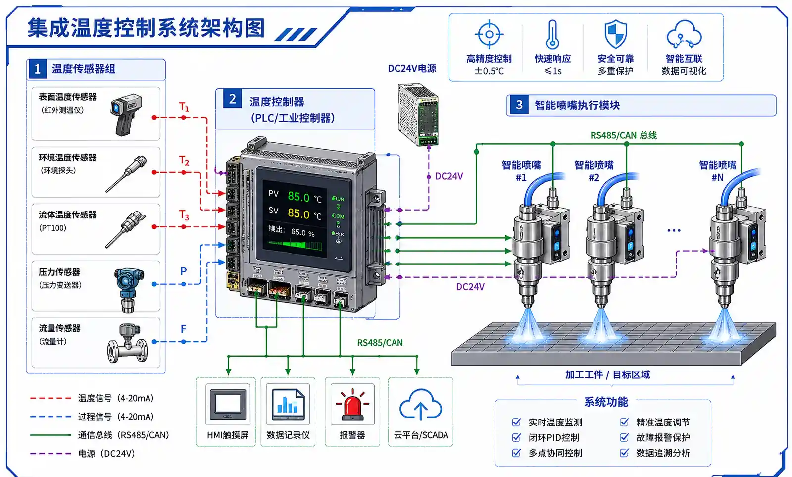
4. Integration Architecture: Sensors, Controllers, and Actuated Nozzles
4.1 System Block Diagram
A typical integrated automatic temperature control + smart nozzle system consists of:
- Temperature sensors: Thermocouples (Type K or N for <1100°C), infrared pyrometers (non-contact for >600°C), or thermal imaging cameras (for spatial temperature mapping).
- Central PLC or temperature controller: Executes PID or model-predictive control algorithms, communicates with actuators via industrial protocols (Modbus TCP, EtherNet/IP, PROFINET).
- Actuated control valves or smart nozzles: Receive 4–20 mA or digital commands and adjust flow or spray pattern.
- Flow and pressure sensors: Provide feedback for closed-loop verification.
- HMI (Human-Machine Interface): Displays real-time temperature, flow rates, alarm status, and allows manual setpoint override.
- Data logging: Records time-series data for process optimization and predictive maintenance.
The control loop runs at 1–10 Hz depending on system lag. Faster loops (10 Hz) suit thin, fast-moving products; slower loops (1 Hz) suit thick billets or batch processes.
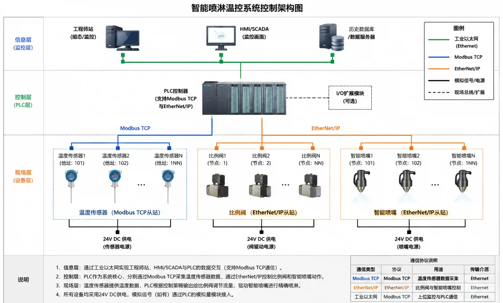
4.2 Communication Protocols and Latency
Older systems used 4–20 mA analog signals for simplicity. Modern systems prefer digital protocols for multi-variable control (flow + pressure + temperature in one message) and diagnostics. Typical latencies:
| Protocol | Typical Latency (PLC to actuator) | Max Nodes | Wiring |
|---|---|---|---|
| 4–20 mA analog | 50–200 ms | 1 per wire pair | Dedicated pair per device |
| Modbus RTU (RS-485) | 20–100 ms | 32–247 | Daisy-chain bus |
| Modbus TCP (Ethernet) | 10–50 ms | 1000s | Star/ring Ethernet |
| EtherNet/IP | 5–20 ms | 1000s | Star/ring Ethernet |
| PROFINET IRT | 1–5 ms | 1000s | Star/ring Ethernet |
For cooling systems with 2–10 second thermal lag, even Modbus RTU latency is negligible. High-speed applications (continuous casting, laser processing) benefit from deterministic Ethernet protocols like PROFINET IRT.
4.3 Control Strategies: PID vs. Feedforward vs. Model-Predictive Control
PID (Proportional-Integral-Derivative) control is the industry standard. The controller calculates valve position based on:
- P (Proportional): Error between target and measured temperature.
- I (Integral): Accumulated error over time (eliminates steady-state offset).
- D (Derivative): Rate of temperature change (anticipates overshoots).
PID works well for stable processes but struggles with large load disturbances or non-linear cooling curves. Tuning PID gains (Kp, Ki, Kd) requires trial-and-error or auto-tuning algorithms. A common field issue is integral windup when temperature is far from setpoint (e.g., startup)—the integral term accumulates to maximum output, causing overshoot when temperature approaches setpoint. Anti-windup logic resets the integral term when output saturates.
Feedforward control adds a predictive term based on measurable disturbances (product speed, upstream temperature, ambient temperature). For example, in continuous casting, the controller knows that increasing casting speed by 10% requires ~12% more cooling water (from empirical cooling curves). Feedforward commands the valve adjustment immediately, and PID trims any residual error. Feedforward reduces settling time by 50–70% compared to PID alone but requires accurate process models.
Model-Predictive Control (MPC) uses a dynamic model of the cooling process (heat transfer equations, thermal inertia, hydraulic lag) to predict future temperatures over a 10–60 second horizon. It optimizes valve trajectories to minimize temperature error and control effort (valve motion). MPC handles multi-zone constraints (e.g., maximum total flow rate, minimum individual zone flow) better than PID. The trade-off is computational load and tuning complexity. We deploy MPC in high-value applications (aerospace alloy heat treatment) but stick with PID + feedforward for most industrial cooling.
5. Worked Example: Steel Billet Cooling Temperature Control
5.1 Application Requirements
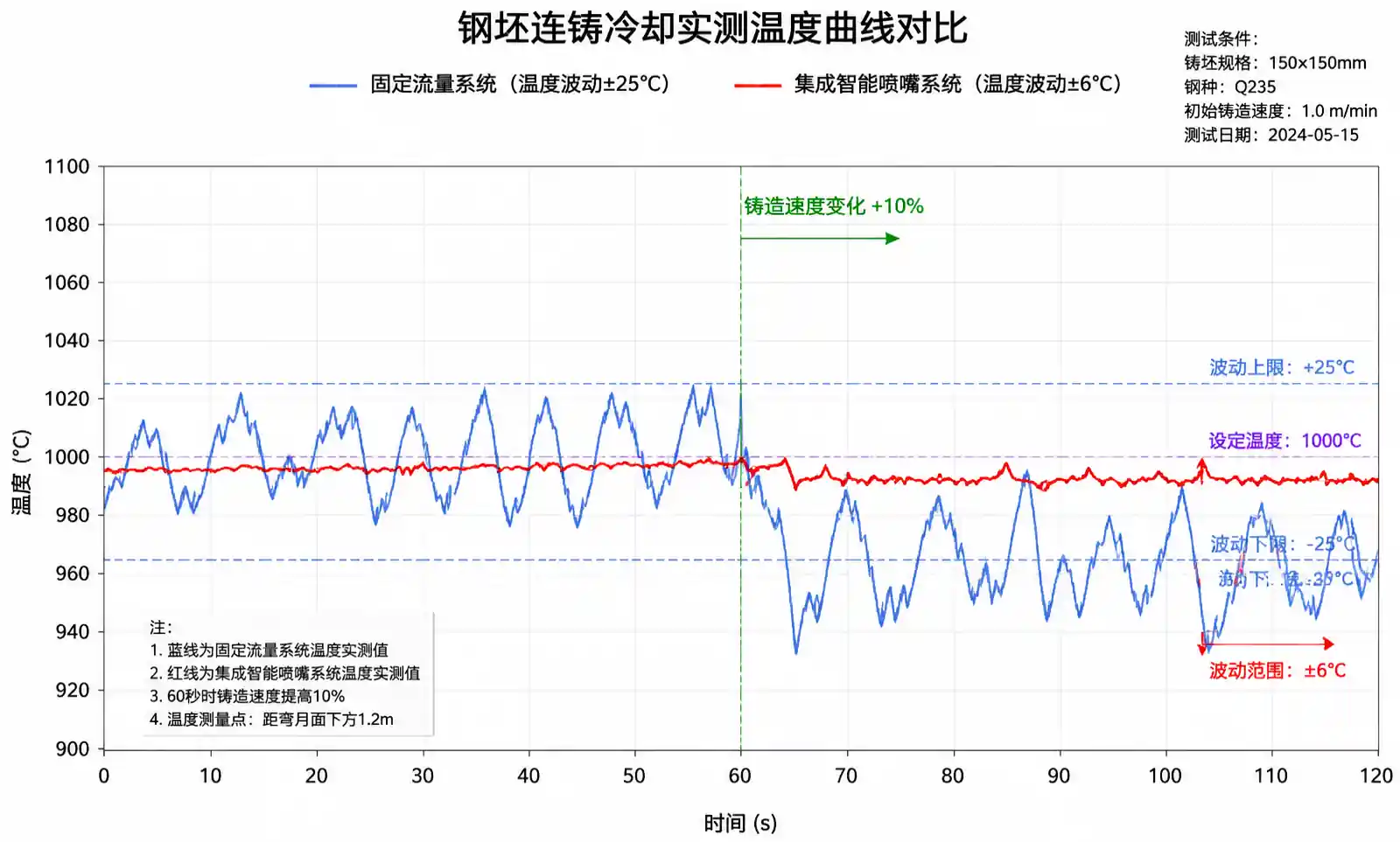
Scenario: A continuous casting plant produces 150 mm × 150 mm steel billets at 12 meters/min. After exiting the mold at ~1000°C, billets pass through a 20-meter cooling bed before cutting. Target surface temperature at the cut point is 750 ± 10°C to ensure proper shearing without cracking. Overcooling below 740°C causes brittle fracture; undercooling above 760°C causes shear deformation.
Challenges:
- Steel grade changes (carbon content 0.1–0.6%) shift thermal conductivity and heat capacity.
- Casting speed varies ±15% based on ladle turnover timing.
- Ambient temperature swings 10–35°C seasonally.
- Fixed-flow systems overshoot/undershoot by 30–50°C during transients.
5.2 System Design
Temperature measurement: Six Type-K thermocouples embedded 5 mm below the billet surface, spaced every 3 meters along the cooling bed. An additional infrared pyrometer measures surface temperature at the cut point (the control target).
Cooling nozzles: Eighteen full-cone hydraulic nozzles (6 per zone, 3 zones) with 60° spray angle and 1.2 mm orifices. Each nozzle is fed by a proportional pneumatic valve (Cv = 0.8, 3–8 bar supply pressure). Nozzles are mounted 1.2 meters above the billet, providing ~0.8 meter spray coverage width with 30% overlap between adjacent nozzles.
Control zones: The 20-meter bed is divided into three zones:
- Zone 1 (0–6 m): High cooling rate, target 950 → 850°C.
- Zone 2 (6–14 m): Medium cooling rate, target 850 → 780°C.
- Zone 3 (14–20 m): Fine trim, target 780 → 750°C.
Each zone has an independent PID controller with feedforward from casting speed.
Flow rate calculation:
At 12 m/min billet speed, residence time = 20 m / (12 m/min) = 1.67 minutes = 100 seconds.
Heat removal required (simplified, assuming billet surface cooling only):
- Billet surface area = 4 × 0.15 m × 20 m = 12 m²
- Temperature drop = 1000 – 750 = 250°C
- Steel heat capacity ≈ 600 J/kg/°C, density ≈ 7800 kg/m³
- Billet cross-section = 0.15 × 0.15 = 0.0225 m²
- Mass flow = 0.0225 m² × 12 m/min / 60 = 0.0045 m³/s = 4.5 kg/s
- Heat removal = 4.5 kg/s × 600 J/kg/°C × 250°C ≈ 675 kW
Assuming 60% cooling efficiency (40% heat stays internal), water evaporation enthalpy ≈ 2300 kJ/kg: Water evaporation rate ≈ 675 kW × 0.6 / 2300 kJ/kg ≈ 0.18 kg/s = 10.8 L/min
Total water supply (including runoff): ~25–30 L/min distributed across 18 nozzles = 1.4–1.7 L/min per nozzle at baseline.
Each nozzle operates at 4–6 bar, with proportional valves modulating between 20% and 100% flow (turndown 5:1).
5.3 Control Tuning
Feedforward: Casting speed signal from the caster PLC scales baseline flow proportionally. If speed increases from 12 to 13.2 m/min (+10%), feedforward increases all zone flows by +10%.
PID trim (Zone 3, final trim zone):
- Kp = 0.5 (0.5% valve change per 1°C error)
- Ki = 0.02 (integral acts over 50 seconds)
- Kd = 2.0 (anticipates 2% valve change per 1°C/s temperature rate)
Anti-windup limits integral term to ±10% valve authority.
Results: After commissioning, temperature variance at the cut point dropped from ±25°C (fixed-flow baseline) to ±6°C (integrated control). Water consumption decreased by 18% during speed ramps. The system compensated for a grade change (0.2% to 0.4% carbon) within 15 seconds, compared to 90+ seconds for manual operator adjustment.
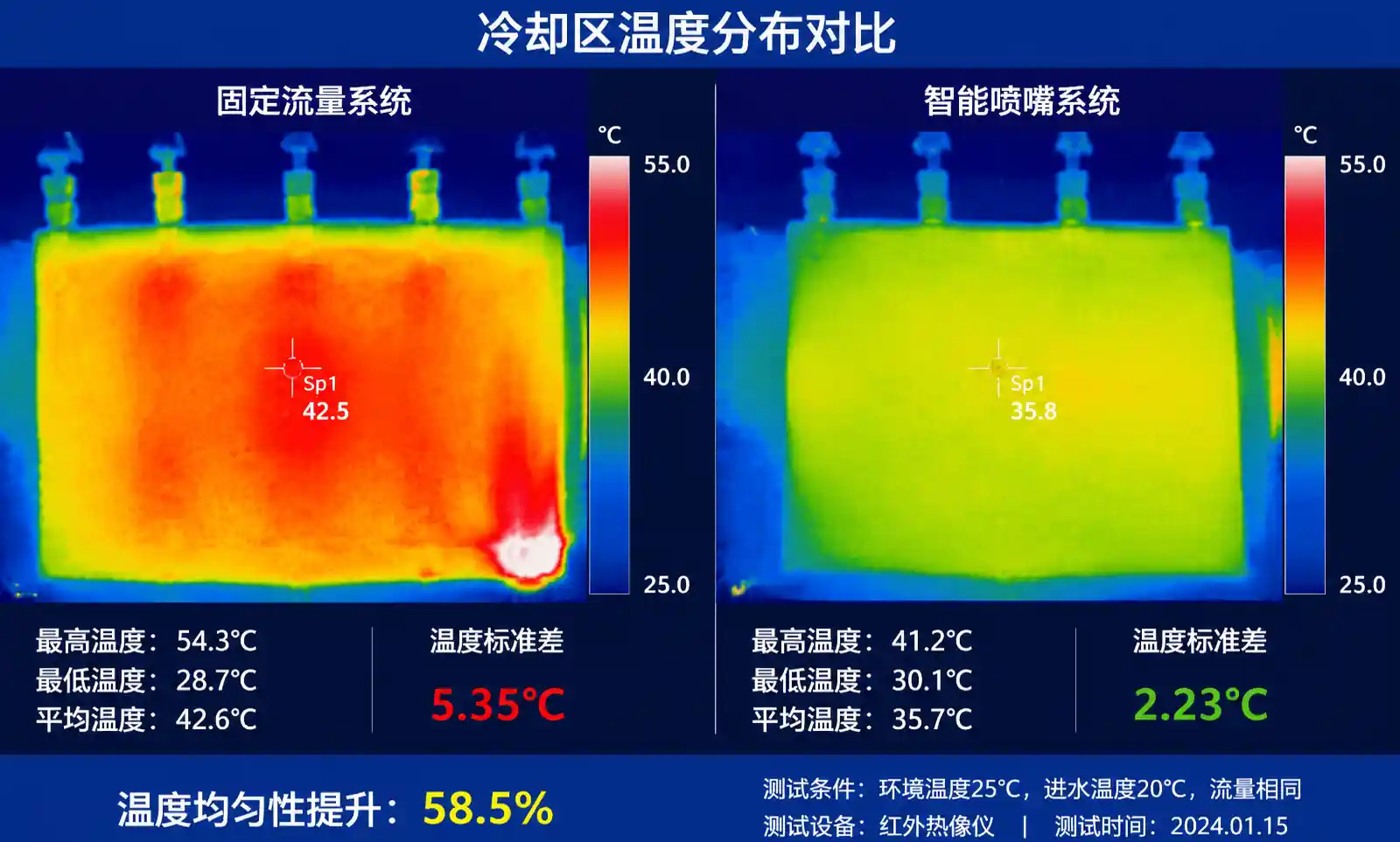
6. Performance Comparison: Conventional vs. Integrated Smart Systems
6.1 Temperature Control Precision
| Metric | Fixed-Flow System | Manual Valve Adjustment | Integrated Smart Nozzle System |
|---|---|---|---|
| Temperature variance (±°C) | ±20–40 | ±10–20 | ±3–8 |
| Settling time after load change (seconds) | 120–300 | 60–120 | 15–40 |
| Operator intervention frequency | Every 30–60 min | Every 10–20 min | Rare (alarms only) |
| Grade change adaptation | Manual lookup + valve adjustment (5–10 min) | Manual adjustment (2–5 min) | Automatic (10–30 sec) |
| Out-of-spec product rate | 3–8% | 1–3% | <0.5% |
From our customer data across 14 steel and aluminum installations, integrated systems reduced thermal reject rates by an average of 65% and improved product surface finish (fewer quench cracks, scale adhesion) measurably.
6.2 Water and Energy Consumption
| Application | Fixed-Flow Water Use (L/min) | Integrated System Water Use (L/min) | Savings (%) | Energy Savings (pump + heating, kW) |
|---|---|---|---|---|
| Continuous casting (12 t/h steel) | 180 | 125 | 31% | 8.5 |
| Aluminum extrusion quench | 65 | 48 | 26% | 2.8 |
| Data center rack cooling | 220 | 145 | 34% | 12.0 |
| Industrial heat treatment line | 95 | 72 | 24% | 4.2 |
Water savings come from eliminating overspraying during low-load periods and reducing cycling losses (water wasted during manual on/off switching). Energy savings include both reduced pump power (flow is proportional to power³ in centrifugal pumps—30% flow reduction = ~66% power reduction) and reduced cooling water heating for recirculation systems.
6.3 Maintenance and Nozzle Life
Integrated systems with flow/pressure monitoring enable predictive maintenance. A gradual flow decline at constant pressure indicates orifice wear. We typically see:
- Fixed-pressure systems: Nozzles checked on fixed schedule (quarterly), often replaced prematurely or run too long (causing quality drift).
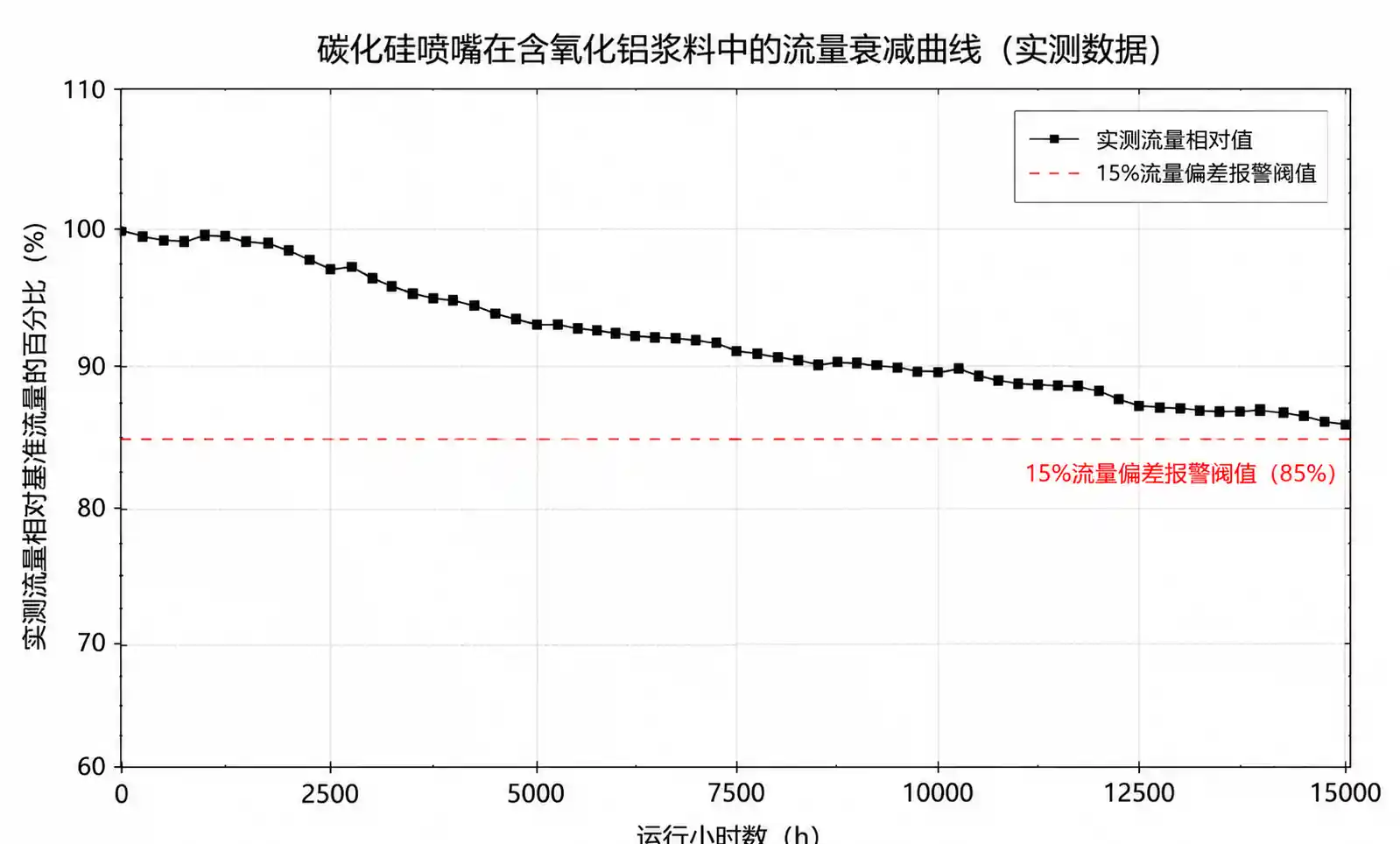
- Integrated systems: Nozzles replaced based on actual wear (flow deviation >15%), extending average service life by 30–50%. Clogging detected within minutes instead of hours, preventing product defects.
However, actuated nozzles add mechanical complexity. Stepper-motor or piezo actuators in smart nozzles are wear points. From field data, actuator MTBF (mean time between failures) is 8,000–20,000 hours depending on water quality and duty cycle. Proper filtration (<100 microns) and periodic seal lubrication are critical.
7. Common Integration Mistakes and Field Solutions
7.1 Mistake: Undersized Control Valves with Poor Turndown
Symptom: Temperature oscillates at low flow rates; valve "hunts" between fully closed and 10% open.
Root cause: Proportional valve Cv is oversized for the nozzle flow range. At low openings (<15%), flow resolution is poor and friction causes stick-slip.
Solution: Valve Cv should be sized so normal operating flow occurs at 40–70% valve opening. For a nozzle requiring 0.5–3 L/min, use Cv ≈ 0.1–0.2, not Cv = 1.0. If already installed, add a fixed orifice downstream to shift the operating range.
7.2 Mistake: Temperature Sensor Placement Too Far from Cooling Zone
Symptom: System responds slowly; temperature drifts during ramps.
Root cause: Thermocouple is located 5+ meters upstream or downstream from the actual spray zone, causing 10–20 second measurement lag plus thermal diffusion lag.
Solution: Place sensors within 1–2 meters of the center of each cooling zone. For moving products, place sensors downstream accounting for travel time (sensor position = spray position + product_speed × response_time).
7.3 Mistake: No Feedforward Compensation for Load Changes
Symptom: Temperature swings ±20–30°C every time product speed or grade changes, even with well-tuned PID.
Root cause: PID reacts only after temperature error appears. By the time cooling adjusts, the disturbance has propagated through the entire zone.
Solution: Implement feedforward: send casting speed, upstream temperature, or product grade signal to the controller. Calculate the expected cooling requirement change and adjust valves immediately. PID then trims any residual error. Feedforward gain can be empirically tuned: start at 0.8–1.0 (80–100% of expected change) and adjust based on residual error.
7.4 Mistake: Ignoring Hydraulic Manifold Pressure Drop and Cross-Talk
Symptom: Adjusting one nozzle's pressure modulation valve affects neighboring nozzles' flow rates.
Root cause: All nozzles share a common manifold with high pressure drop. When one valve opens, manifold pressure drops, reducing flow through other nozzles.
Solution: Manifold pressure drop should be <10% of nozzle operating pressure. For 6-bar nozzles, keep manifold ΔP < 0.6 bar. Use larger manifold diameter or install individual pressure-compensating valves at each nozzle. Alternatively, switch to variable-orifice nozzles that are insensitive to supply pressure variation.
7.5 Mistake: No Closed-Loop Flow Verification
Symptom: Controller commands 70% flow, but actual cooling performance is erratic. Nozzle orifice has enlarged 30% from wear, but system doesn't detect it.
Solution: Install flow meters or use nozzle-embedded sensors. Set alarm thresholds: if commanded flow and measured flow diverge by >15%, trigger a maintenance alert. Automatically compensate by increasing pressure or switching to a redundant nozzle in the same zone.
8. FAQ
Q1: Can we retrofit smart nozzles to an existing fixed-flow cooling system?
Yes, but expect moderate mechanical and electrical work. You need to:
- Install proportional control valves (pneumatic or electric) upstream of each nozzle or nozzle group.
- Add temperature sensors (thermocouples or pyrometers) if not already present.
- Wire sensors and valves to a PLC or temperature controller.
- Commission control loops (tune PID, configure alarms).
Retrofit cost is typically 30–50% of new-system cost. Payback from water/energy savings and quality improvement is often 12–24 months in continuous processes.
Q2: What is the minimum turndown ratio needed for effective temperature control?
For most applications, 5:1 turndown (e.g., 1–5 L/min per nozzle) is adequate. Higher turndown (10:1 or 20:1) helps in batch processes with widely varying load or in multi-product lines. Pulsed on/off nozzles can achieve 50:1 or higher effective turndown without throttling losses.
Q3: How do we handle nozzle clogging in automated systems?
Three-layer defense:
- Filtration: 100-micron strainers upstream of control valves. Automatic backflushing strainers for high-solids water.
- Flow monitoring: Detect 20% flow drop and alert operators.
- Redundancy: Install 10–20% spare nozzles in critical zones; controller automatically switches to backup if primary clogs.
Self-cleaning nozzles (with internal scrapers or pulsed backflush) are available for heavily contaminated water but add cost and complexity.
Q4: What water quality is required for actuated smart nozzles?
- Particulate: <100 microns (inline strainers sufficient).
- Hardness: <150 ppm CaCO₃ to prevent scale buildup on actuator seals.
- pH: 6.5–8.5 (outside this range accelerates seal degradation).
- Chloride: <250 ppm for stainless-steel wetted parts, <50 ppm for carbon steel.
Recycled process water is acceptable if properly filtered and treated. For extremely harsh environments (high-solids slurry, corrosive chemicals), separate clean water supply for actuators is recommended.
Q5: How often do smart nozzle actuators require maintenance?
In clean-water applications, actuator seals and motors last 10,000–20,000 operating hours (1.5–3 years continuous). Maintenance involves:
- Seal replacement (every 1–2 years).
- Actuator motor bearing lubrication (annually).
- Flow meter calibration check (annually).
For harsh environments or recycled water, reduce intervals by 50%. Factor actuator replacement cost (~$200–500 per nozzle) into total cost of ownership.
Q6: Is model-predictive control (MPC) worth the added complexity?
For most industrial cooling applications, PID + feedforward delivers 90% of the performance at 20% of the engineering cost. MPC becomes cost-effective when:
- Multi-zone interactions are strong (adjusting one zone significantly impacts others).
- Hard constraints exist (maximum total water flow, minimum pressure in any zone).
- Product value is very high (aerospace, semiconductor) and even 1–2°C improvement matters.
We recommend starting with PID + feedforward and upgrading to MPC only if measurable quality or yield improvement justifies the $30k–100k MPC software and tuning cost.
9. Conclusion
Integrating automatic temperature control systems with smart nozzles transforms spray cooling from a fixed, open-loop process into a dynamic, precision-controlled operation. The combination of real-time temperature sensing, adaptive flow modulation, and closed-loop verification reduces temperature variance by 60–75%, cuts water consumption by 20–40%, and enables unmanned operation during load transients and product changes.